Overview
In this supplemental module, you will perform a parametric transient analyses of an inverter using a test-bench circuit. The objective is to determine the width of the NMOS and the width of the PMOS such that the response is close to symmetric. Moreover, both the rise and fall times should be less than 100 ps.Basic setup
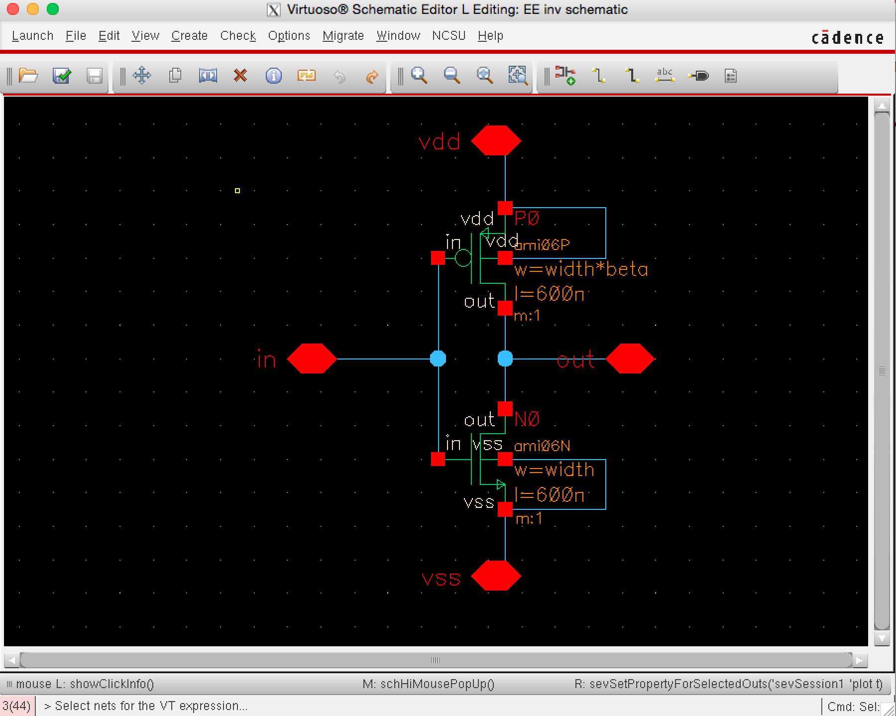
Create a new schematic called "pinv". Create the standard schematic for an inverter. In the schematic, let "width" be the width of the NMOS, i.e., enter the string "width" in the width property field of the NMOS. Let "width*beta" be the width of the PMOS. The result is shown below.
Create a test-bench with a 10fF load as described in the previous tutorial and open up the ADE simulation environment. Perform the basic setup as described in the earlier module explaining transient analysis. (At this point, you will not have the "Design Variables" shown to the left and you will only have two outputs. In the next part, it will be explained how to enter/obtain these "missing" values.)
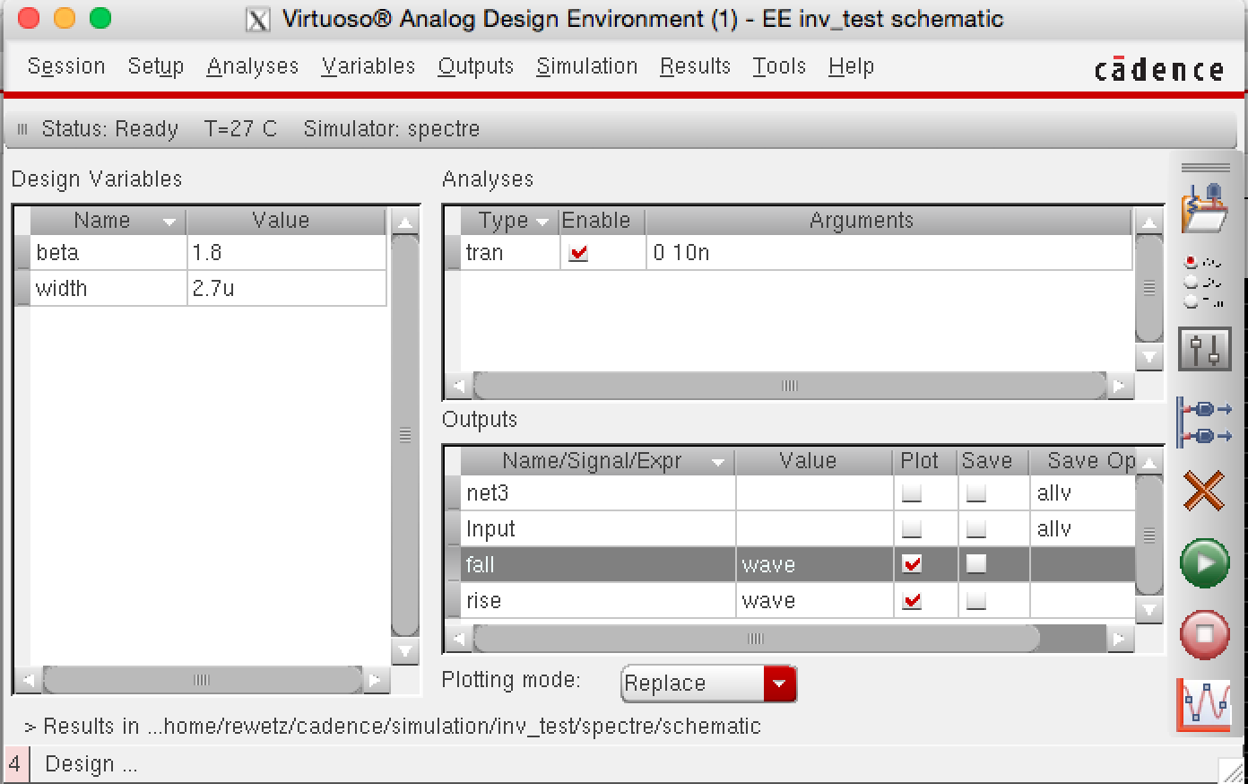
Next, press "Variables" and select "Add from Cellview". As a result, the Design variables "beta" and "width" will appear in the left side of the window as illustrated in the figure, above. Set beta to "1" and width to "1.5u" (in the figure beta=1.8 and width=2.7u). Using the parameters, it is easy to perform various simulations.
Setup of outputs using expressions
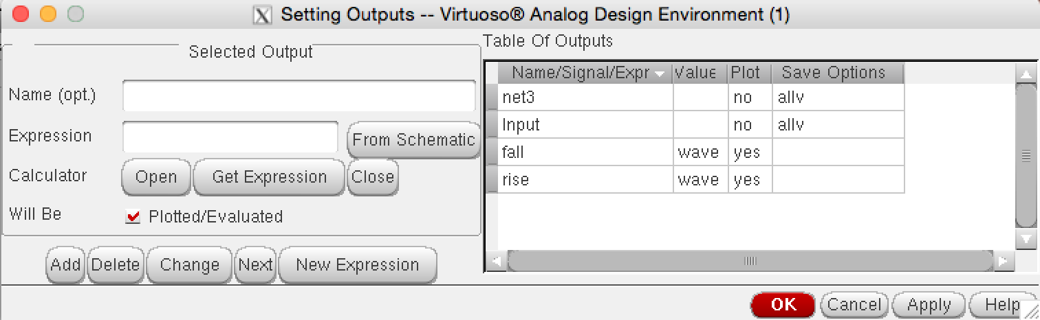
In the previous tutorial, the output waveform of the inverter was plotted and the rise and fall times were computed from the plots. However, it is rather tedious approach. In the next step, it will be demonstrated how to add an output variable storing the numeric value of the rise or fall time, i.e., the two additional outputs, denoted "fall" and "rise" as shown in the figure above.Double click on one of the current outputs. This will open the "Settings Outputs" window. Press the "Next" button and an empty form for a new output will be displayed, as shown below.
Set the "Name (opt)" field to "rise". Next, the expression for the rise-time will be specified. (This is slightly more complicated than obtaining the expression for the output voltage (in the earlier module), which was simply obtained by clicking on the net using the "From Schematic" button.) To generate the "expression" for the rise time, open the calculator by pressing the "Open" button. The calculator window below will open.
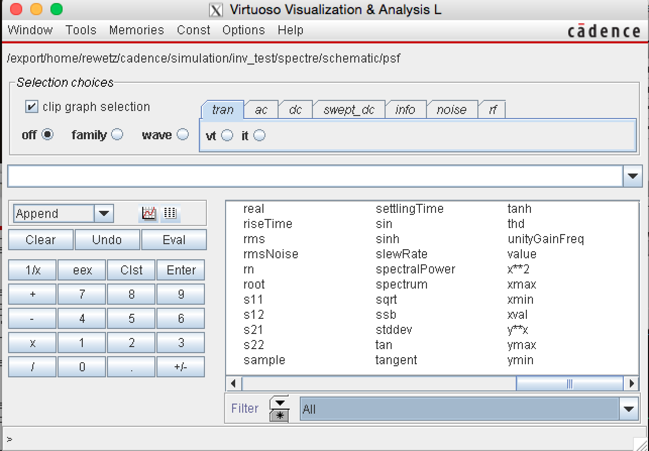
Select riseTime from the alternative functions in the bottom right. The following form will appear.
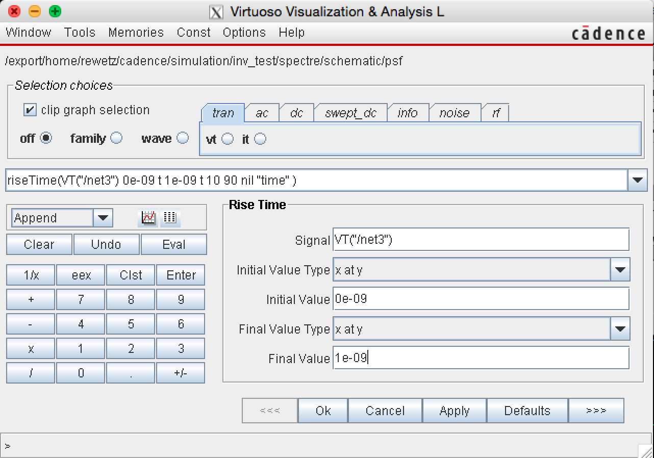
Fill out the values as shown in the figure (do not enter the "riseTime(VT....)" string, it will be generated for you). In the example, "net3" is the name of the output net/wire of the inverter in the test schematic. The "Initial value" and the "Final value" should be set to encapsulate a single rising or falling transition. Based on the input signal, we know that there is a rising transition in the "0" to "0e-09" (or 1 ns) interval. (When generating the expression for the fall time, fill out the form in the same manner but set the Initial value to "1e-09" and the Final value to "2e-09".)
After you have completed the form, press "Ok", and the expression "riseTime(VT(....)" will be generated in the calculator. Next, return to the "Setting Outputs window" and press "GetExpression". This will copy the generated expression from the calculator to the "Expression" field. Repeat the same process for the output called fall. Use the riseTime function but a different time interval. (The riseTime function is used to compute both falling and rising transitions.)
Next, perform a simulation by pressing the green play button called "Netlist and Run". The values of the rise and fall times for the given width and beta parameters will be computed and displayed as numeric values.
Parametric sweep
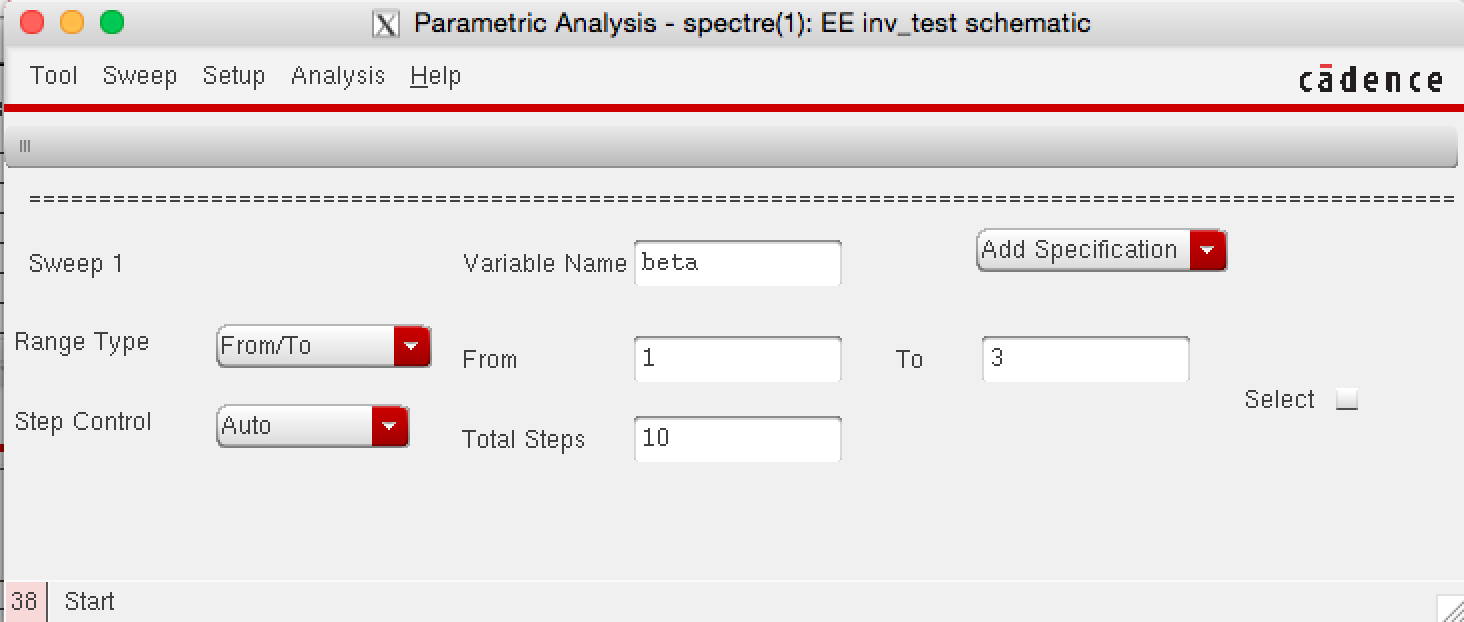
Instead of manually trying to find parameter values for "beta" and "width" that satisfy the specification requirements, a parametric sweep can be performed. Basically, a sweep variable is selected and the fall and rise time will be computed for various values of that sweep variable.To perform a parametric sweep, select Tools->Parametric Analysis. The window shown below will be opened, select beta as the "Sweep 1" parameter and fill out the form accordingly.
Next, press Analysis->Start in the Parametric Analysis window. This will plot the rise and fall times as a function of beta, as illustrated below.
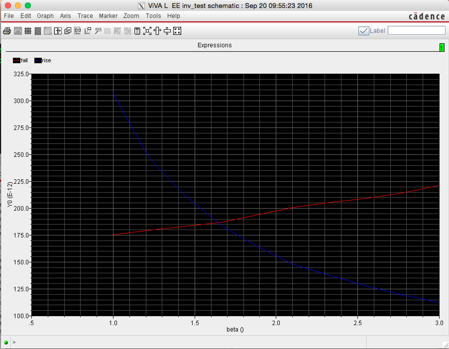
As expected, the fall time increases and the rise time decreases when "beta" is increased. Select a "good" value for beta (set the Design parameter beta to this "good" value in the main window) and repeat the sweep for the "width" parameter. This will result in a plot similar to as follows.
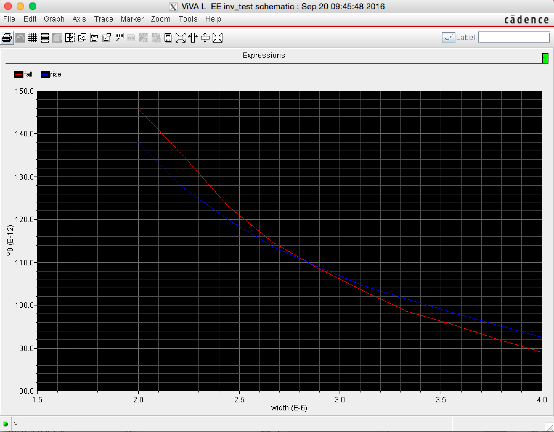
By selecting the width to be 3.5u, both the rise and fall times will be below 100 ps. From the figure it can be observed that the rise and fall time difference is small. However, using the new width, it is possible to sweep the "beta" parameter again, to further improve performance.